1976
A frontier model passes every run on my hardest geometry task and loses to a spring written down fifty years ago; the distance between the two is a ladder, and every rung hides one more layer of machinery.
Fourteen for fourteen, then a spring
I build CAD and simulation environments that frontier models train against, for Anthropic. The hardest geometry task I have shipped is a B-rep1 retrieval problem where up to half the part has been torn away. Fable 5 passes every run of it. Against a mass-spring model published in 1976, the same model fails 85% of the time.
I pulled 1,758 scored rollouts from our training infrastructure to see whether that was a fluke. It is a staircase. Group the tasks by what they ask the model to do and the pass rate falls one step at a time. What each step measures is precise: how much machinery sits between what the model observes and what generated it. Each rung down hides one more layer.
24 problemsclassify, retrieve, rank geometry
14 problemsforecast a field you can watch
19 problemspredict the solver's output from geometry
20 problemsrecover the mechanism from its response
no problemsproduce the part itself
This essay walks the ladder rung by rung, with the actual tasks, the actual reward code and the actual physics, down to the spring at the bottom and the empty rung below it.
01 See
The answer is a property of what you can look at. 50% pass
Start at the top, where models are frighteningly good. These tasks hand the model geometry and ask a question whose answer is a function of that geometry: classify the surface type, rank the catalog, find the part.
My retrieval task lives here. Take a real CAD body from the Autodesk Fusion 360 Gallery. Rotate it randomly in SO(3), rescale it by a factor drawn from U(0.5, 2.0), jitter every surface point, tear away up to 55% of its faces keeping only the largest connected piece, shuffle what remains. Then ask the model to find the original in a gallery of 180 bodies.
The model never sees a solid. Each face is downsampled to a 5×5 grid of surface samples2, stacked into a tensor, with an adjacency graph saying which faces touch:
# environment/corrupt.py · shipped to the agent in full
def corrupt(graph, *, seed, dropout_low, dropout_high):
    """Return an independently corrupted view of ``graph``.

    Applies, in order: a uniform random SO(3) rotation of surface
    points and normals, a global rescale in U(0.5, 2.0), masked
    Gaussian jitter of points and normals, connectivity-grown face
    dropout keeping the largest connected component, and a random
    face permutation with shuffled edges."""
    # uv_grid:    [F, 5, 5, 7]  (xyz, unit normals, coverage mask)
    # edge_index: [2, E]        (face adjacency)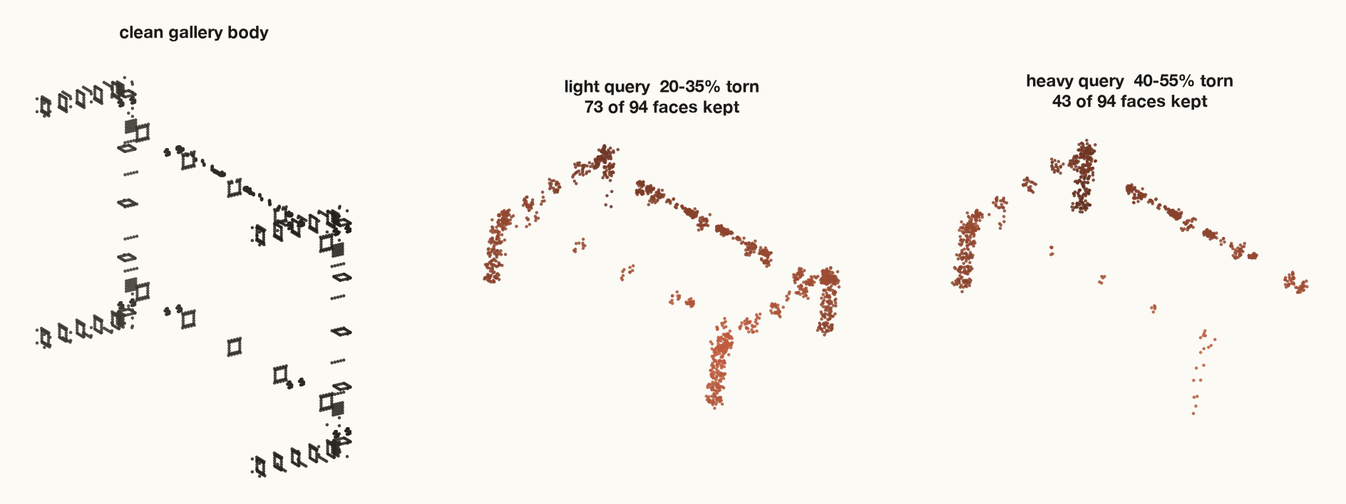
This should be hard. It is not. Fable 5 passes 14 of 14 runs on this task with a mean reward of 0.95, and the whole rung sits at 50%, with the failures concentrated in a few pathological ranking tasks. The reason defines everything below: the answer here is a stable function of visible structure. Invariance to rotation, scale and occlusion is exactly the regularity a large model extracts from data without ever needing to know what a face or a solid is.
So the corpus takes the first thing away. What if the answer is not a property of the shape but a field that lives on it, produced by machinery the model can watch but not touch?
02 Advance
You can watch the mechanism run. Continue it. 42% pass
The forecasting tasks give the model frames of a physical field, buoyancy and velocity in a convecting fluid, density and magnetic field in a turbulent plasma, and ask it to advance the state several steps in one shot. The mechanism is fully visible; every frame is the mechanism operating. The model has to continue what it can already see.
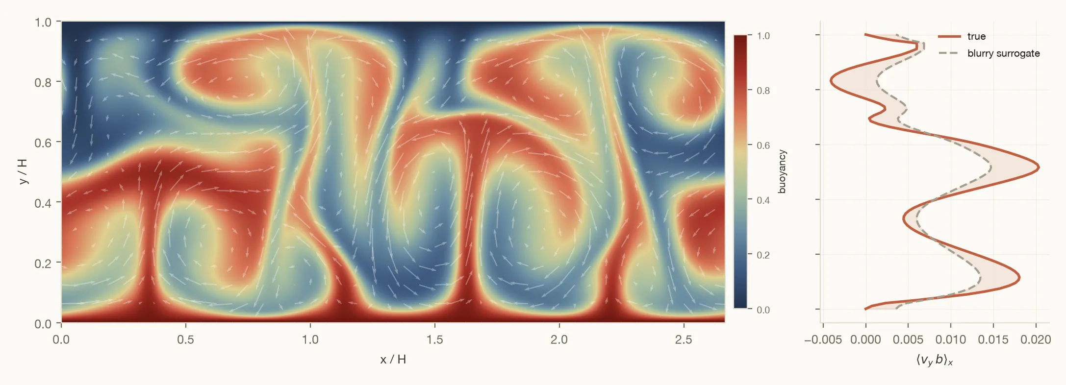
Pass rate: 42%. The dominant failure is the one every pixel-loss model commits: blur. Averaging over plausible futures minimises mean squared error and produces a fluid that has stopped obeying physics, plumes smeared into gradients, sharp fronts gone. The per-pixel numbers still look respectable. That is why these tasks never grade the field alone. They also grade a derived invariant the physics must satisfy, one a blurry field gets wrong:
# rb-nusselt-forecast · the reward gate
# F(y) = <v_y * buoyancy>_x -- the convective heat flux profile.
# A nonlinear diagnostic of the *coupling* between fields: blurring
# v_y and b separately destroys their correlation, so MSE-minimising
# forecasts fail here even when per-pixel error looks fine.
reward = min(gate(field_rel_l2), gate(heatflux_rel_err))
The min is the house style of the entire corpus and we will meet it again. Notice what still makes this rung passable: the model is shown the operator in action. Two context frames of a convection cell carry an enormous amount of what it needs. The next rung deletes those frames.
03 Produce
You never see the field. Produce what the solver would say. 18% pass
Here the model receives only geometry, a jet-engine bracket as a point cloud or a voxel grid, and must output what a finite-element solver would compute on it: the von Mises stress3 field under load, the displacement field, the first vibration mode. It has training pairs, geometry in and field out, but it never observes the operator connecting them. The physics has moved behind a curtain.
Take the first four vibration modes of a bracket section, out of an eigenvalue solve. The dark curves are nodal lines4, where the part does not move at all. Ribs and cut-outs set their position, they migrate as the design changes, and a model that blurs them has produced a physically meaningless answer that still scores well on mean squared error.
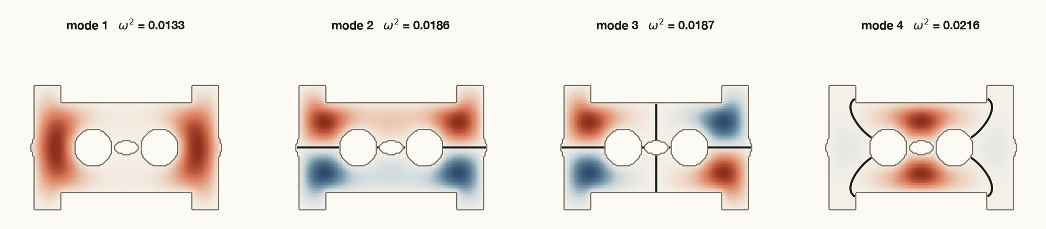
Pass rate 18%, less than half the rung above. The failures now come in a second flavor beyond blur: degenerate specialisation. Predict the easy component of the answer perfectly, abandon the rest, collect partial credit. On one bracket task, mass is nearly a linear function of occupied volume, so a model can nail it from the voxel count alone while ignoring stress and frequency, and an averaged reward would pay it for that.
This is why every task on the rung grades several metrics and takes the minimum, with each metric mapped through four measured anchors. Here is the scoring function from my retrieval task's verifier, verbatim, and it is the same shape everywhere in the corpus:
# tests/verify.py · the reward
def _metric_reward(value, baseline, threshold, target, strong):
    if value <= baseline:  return 0.0
    if value < threshold:  return 0.2 * _smoothstep((value - baseline) / (threshold - baseline))
    if value < target:     return 0.2 + 0.3 * _smoothstep((value - threshold) / (target - threshold))
    if value < strong:     return 0.5 + 0.5 * _smoothstep((value - target) / (strong - target))
    return 1.0

# reward = the WORST metric, not the average. A model that solves
# one third of the problem perfectly scores zero, not one third.
reward = max(0.0, min(1.0, min(scores.values())))
The anchors are measurements, not aspirations. baseline is what an untrained network actually scores. target is where the trained reference solution actually lands. Below is that function running on the real anchors shipped in my task. Try to find a setting where being excellent at two of three metrics pays.
Arrow keys move the metric. The reward below is the lowest of the three scores.
Exactly at the reference solution: every metric on its target anchor.
So far the hidden thing has been an output: a field the model must reproduce. The operator producing that field was fixed and universal, the same elasticity everywhere, the same heat equation. One rung further down, the hidden thing is the operator itself.
04 Invert
The spring. 15% pass
In 1967 Robert Bouc wrote down a differential equation for hysteresis5, the property by which a material's restoring force depends not on where it is but on where it has been. In 1976 Yi-Kwei Wen extended it into the form every earthquake and vibration engineer now knows, and the Bouc–Wen oscillator became one of the standard benchmarks for nonlinear system identification6. It is five lines of physics:
# the Bouc–Wen hysteretic oscillator · from the task's reference solution
# m*y'' + c*y' + k*y + z = u(t)
# z'  = a*y' - bg*|y'|*|z|**(nu-1)*z - bd*y'*|z|**nu
#
# z is the hysteretic force: an unmeasurable internal state whose
# value depends on the entire history of the motion. Identified
# benchmark parameters: m=2, k=5e4, a=5e4, bg=800, bd=-1100, nu=1.
def drv(y1, y2, z, uv):
    dz = a*y2 - bg*abs(y2)*abs(z)**(nu-1)*z - bd*y2*abs(z)**nu
return y2, (uv - c*y2 - k*y1 - z)/m, dzThe tasks on this rung hand the model one recording, force in and displacement out, sampled at 750 Hz, and ask it to predict the displacement for a new force record. Nothing else. To do that you have to recover the mechanism: not fit the wiggle, but figure out what kind of machine is wiggling. There are twenty variants in the corpus, contaminated sensors, closed-loop feedback, asymmetric stiffness, thermal drift, and across 520 rollouts the pass rate is 15%, the worst of any family. The single hardest variant, identification from outlier-contaminated data, has a mean reward of 0.04.
Why does this kill a model that shrugs off half-destroyed CAD bodies? Because the training record genuinely does not pin down the mechanism, and pattern-matching has nothing to grab. I can show you. I fit a second oscillator, an impostor whose hysteresis parameters differ from the true ones by a factor of nine and whose exponent is 1.5 instead of 1.0, a physically different machine, so that its response to the training force matches to within 3.5%. Spring A is the benchmark mechanism. Spring B has bg = 91 instead of 800, bd = −117 instead of −1100, ν = 1.5 instead of 1.0. At the training amplitude their responses are 3.5% apart, inside the task's measurement-noise floor. Drive the same two springs 3.5× harder and they disagree by 16%, because the hysteresis terms that were barely excited at small amplitude now dominate.
Every fit that stops at "matches the training data" has a large family of impostors to choose from, and gradient descent will happily pick one. The graders on this rung are built to drive the system into the regime where impostors die: held-out records at higher amplitudes, different spectral content, reversed sweeps. That is not adversarial cruelty. It is the definition of having identified a system.
You can run the experiment yourself. Both springs below are integrated live in your browser with RK47 on the equations above. At drive level 1.0× they are the same spring for all you can tell. Turn it up.
Arrow keys change the drive amplitude. Both springs are re-simulated and the disagreement below updates.
This is what "the model must reason about mechanism" means, concretely. There is no invariance to learn and no smooth map from input to output. The information that separates the true spring from the impostor is not in the training data. It is in knowing which experiment would separate them, which is a physicist's move, not a pattern-matcher's. That is the skill these 520 rollouts are teaching, one failed attempt at a time, and the per-variant scores say the teaching is uneven: the model already passes half its runs on the thermal-drift variant, and almost none on the contaminated one.
The spring is not hard because it is complicated. It is hard because it keeps its mechanism where the data cannot see it.
05 Design
The rung that is not there. absent
Follow the ladder's logic one step further. Rung 3 hides the field. Rung 4 hides the mechanism. Rung 5 hides the artifact itself: here is a load case, a material budget and a manufacturing process, produce the part. That is the job a mechanical engineer is actually paid for, and it is almost completely absent from the corpus. Not because we cannot grade it. Because we cannot afford to.
We have known how to solve the toy version without any learning since the nineties. I ran one while writing this: topology optimisation8 of a beam, nothing given but a load, a support, and permission to use half the material.
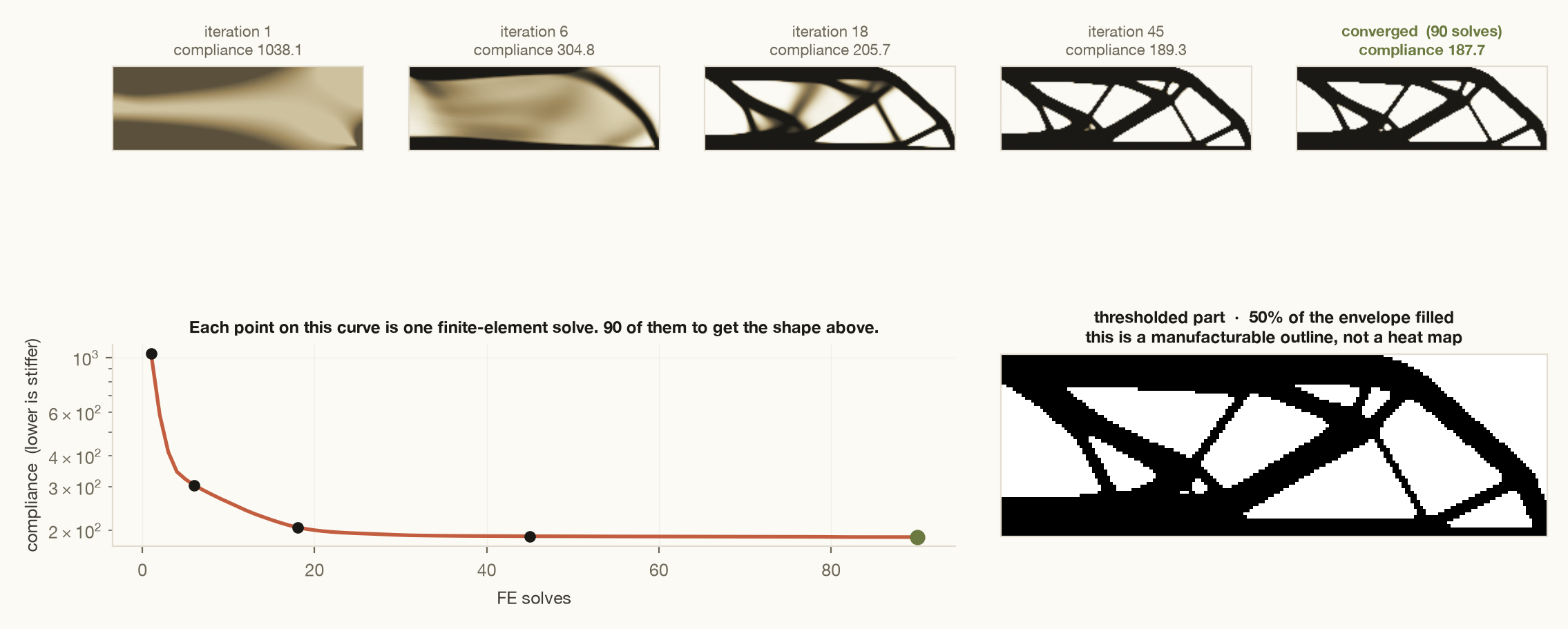
# the whole generative-design loop, in one update
for it in range(90):
    U  = solve(K(x), F)                                  # one finite-element solve
    dc = -penal * x**(penal-1) * strain_energy(U)
    x  = optimality_criteria(x, filter(dc), volfrac)     # move material toward strain
Ninety solves for a two-dimensional, linear-elastic, single-load, compliance-only toy, each solve a few milliseconds. The real version, a 3D bracket, four load cases, a stress constraint, a modal floor, a machinability check, is thousands of solves at minutes each. Grading one design attempt costs more than training on ten thousand prediction tasks, so the prediction tasks are what exist.
There is one place in the corpus where a live solver does sit inside a task: a PCB layout problem whose container ships a real heat-equation solver. It is the exception that shows what the rung would feel like.
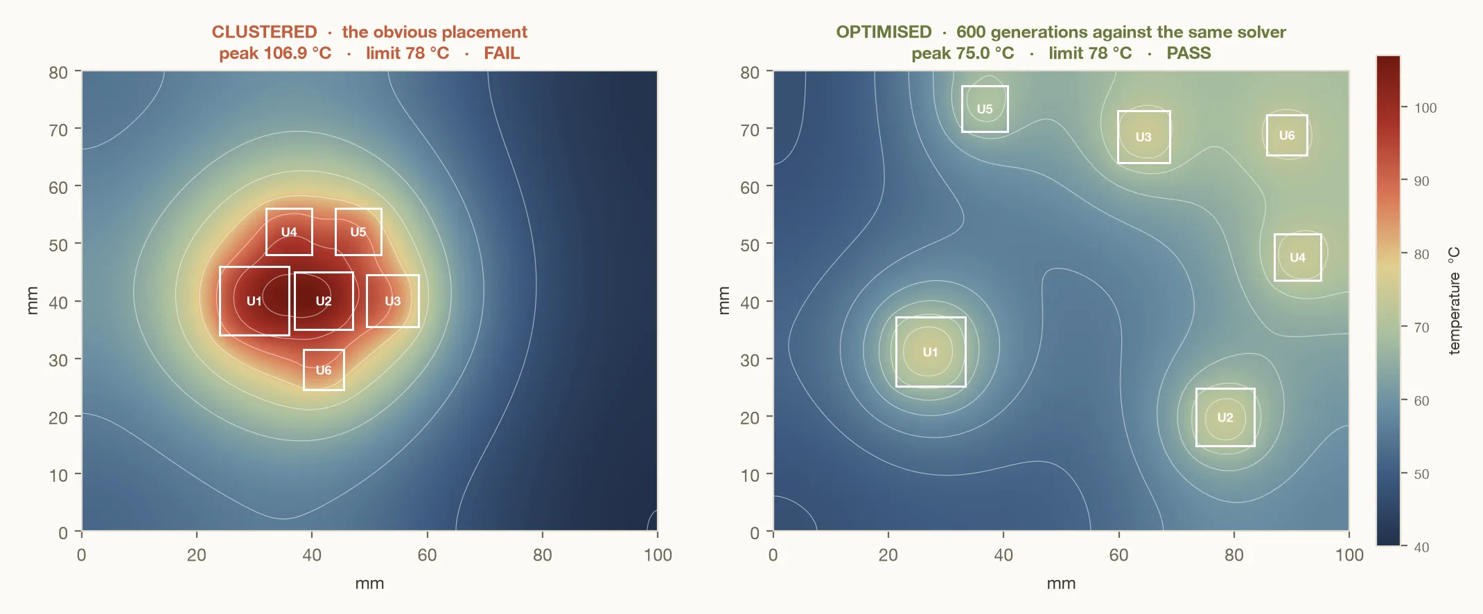
This is why I think the most important number in this field is not a benchmark score but solver latency. Every order of magnitude off the solve time, GPU-native FEM, reduced-order models, surrogates audited by the real solver, moves tasks from "we grade one checkpoint at the end" toward "the agent checks itself a thousand times before submitting", and moves the corpus from prediction toward design. The models are learning physics on rungs 1 through 4 so that they can eventually be trusted as the fast solvers inside rung 5. The ladder eats itself, in the good way.
What the ladder is for
One honest caveat, two hard numbers, then the point.
The caveat: pass rates measure the tasks as much as the model. Task authors set difficulty anchors by hand, and about a third of the variance in per-problem scores traces to which family the task belongs to rather than anything about physics. My own retrieval task is the cautionary example. I calibrated its targets against the frontier in May; by July the model passes every run at a mean of 0.95. The anchors did not get easier. The model got better, which is the entire purpose, and it means the staircase in Fig. 01 is a photograph of a moving object.
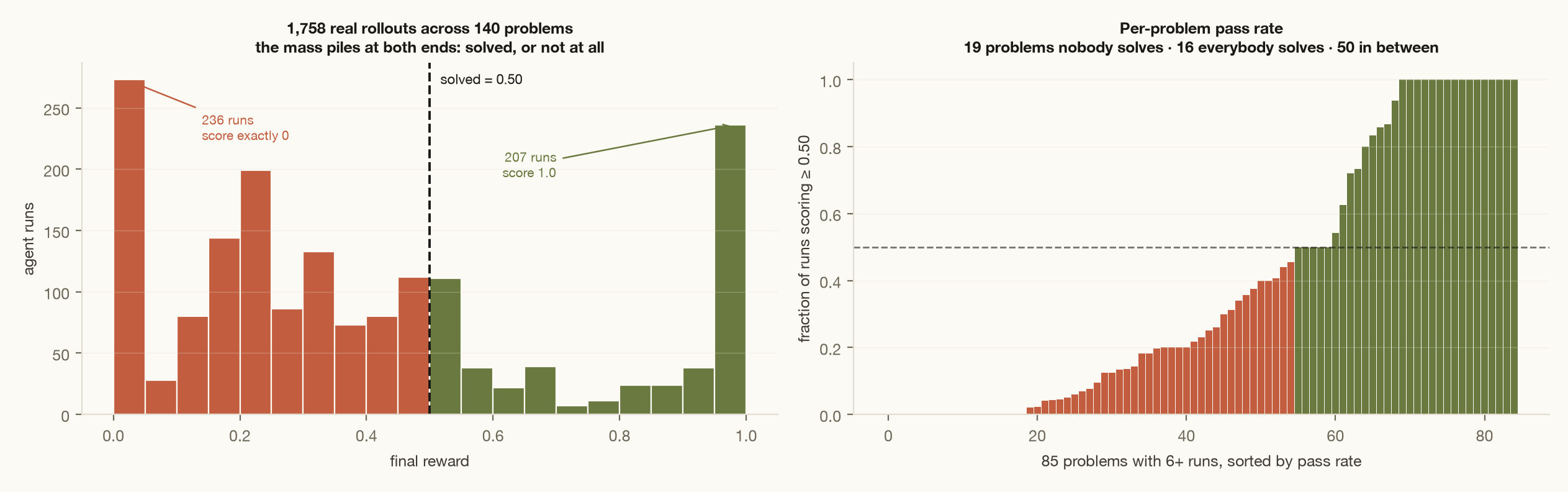
The two numbers. Across all scored rollouts, the correlation between the turns an agent spends and the reward it earns is −0.08. Thrashing is not progress; whatever separates a 0 from a 1 on these tasks is decided early, in whether the model recognises which rung it is standing on. And 23% of runs never produce a score at all, which is a reminder that before any of this gets philosophical, it is infrastructure.
The point. Software taught models to code by giving them a compiler: a verifier that is instant, deterministic, and impossible to argue with. Engineering has something better, physics itself, but its verifiers are slow, so the first generation of physics training looks like this ladder: verify cheap things about expensive simulations. The staircase shows that the cheap-to-verify skills are nearly saturated and the expensive ones, mechanism, inversion, design, are where the frontier actually is. The model that closes the gap on rung 4 will not do it by fitting wiggles better. It will do it the way Wen did in 1976, by knowing what the inside of the machine must look like for the outside to behave the way it does.
Fifty years is a long time for a spring to stay undefeated. I do not think it gets another ten.
Notes
- B-rep: boundary representation, the native format of CAD kernels. A solid described by its faces, edges and vertices and the analytic surfaces they lie on, rather than by a mesh or a voxel grid. ↩
- UV-grid: a fixed-size sampling of a CAD face, surface points and normals evaluated on a regular grid in the face's own parameter space, so that every face becomes the same-shaped tensor regardless of its geometry. ↩
- von Mises stress: a scalar summary of the full stress tensor used to predict yielding. It is the quantity engineers actually contour-plot when they ask whether a part will fail. ↩
- Nodal line: a curve on a vibrating structure that does not move in a given mode. Its position is set by ribs, cut-outs and boundary conditions, and it migrates when the design changes. ↩
- Hysteresis: memory in a mechanical system. The restoring force depends on the deformation history rather than the current displacement alone, so the force-displacement curve encloses a loop instead of retracing a line. ↩
- System identification: recovering a dynamical model, both its structure and its parameters, from measured input-output records. The Bouc–Wen benchmark is a standard test case for the nonlinear version of the problem. ↩
- RK4: the classical fourth-order Runge–Kutta integrator, four derivative evaluations per time step. The in-browser springs integrate the oscillator with it at 6,000 steps per second. ↩
- Topology optimisation: finding where material should exist at all, not just how to size it. SIMP, the standard scheme, gives every element a density between 0 and 1 and penalises the in-between values until the layout resolves into solid and void. ↩
Built for Anthropic as RL training environments for the Claude models; rollout statistics pulled from the training infrastructure in July 2026 (2,293 problem runs, 140 problems, almost all Fable 5). Every figure was computed for this essay: the corruption and retrieval data from the shipped task, the convection panel by explicit Boussinesq integration, the mode shapes by eigensolve, the impostor spring by simulation-error least squares on the Bouc–Wen equations (RK4, 750 Hz record, band-limited forcing), the topology run by SIMP validated against the published MBB benchmark, and the in-browser springs integrate the same ODE live. Datasets: Fusion 360 Gallery (opens in a new tab), DeepJEB (opens in a new tab), the Bouc–Wen identification benchmark (opens in a new tab); encoding after UV-Net (opens in a new tab). R. Bouc, 1967; Y.-K. Wen, Method for random vibration of hysteretic systems, J. Eng. Mech. Div., 1976. Most tasks referenced are other authors' work in the same corpus.